Clustering the MNIST dataset via semidefinite programming

The dataset

The MNIST dataset consists of thousands of images of handwritten digits. (Place the mouse on top of the points in order to see how they look like). The objective is to cluster them by similarity, the previous step for classifying them.

Preprocessing using TensorFlow

Clustering the raw data gives poor results (due to 4’s and 9’s being similar, for example), so we first learn meaningful features, and then cluster the data in feature space. We used the first example from the TensorFlow tutorial. We train a simple one-layer softmax neural network on images from a training set. And we run the trained neural network on the first 1000 elements of the testing set. As a results, each image gets mapped to a $10\times 1$ vector, representing the probabilities of being each digit. Since the entries of the vector sum to 1, the feature space is actually 9-dimensional. Note that spectral clustering would be useless in this case since all its ‘denoising’ comes from projecting the points into the $k-1$ dimensional space spanned by the top $k-1$ eigenvectors of the Laplacian.

These $10\times 1$ feature vectors are the ones we represent in our plot. Since 10 is too many dimensions for a plot, we depict the feature vectors projected onto a random plane.

The k-means semidefinite relaxation

Given a set of points $x_1,\ldots x_n$, the $k$-means objective is to find a partition in $k$ clusters $A_1,\ldots, A_k$ that minimize the sum of the squared distances of the points to the centroid of their respective cluster. In other words,

$$\arg\min_{A_1,\ldots, A_k} \sum_{t=1}^k \sum_{x_i \in A_t} \|x_i - c_t\|^2 \quad \text{where } c_t=\frac{1}{|A_t|}\sum_{x_i\in A_t}x_i.$$

The k-means SDP is based on the following observation:

$$\sum_{t=1}^k \sum_{x_i \in A_t} \|x_i - c_t\|^2 = \frac12\sum_{t=1}^k \frac1{|A_t|} \sum_{x_i\in A_t}\sum_{x_j\in A_t}\|x_i-x_j\|^2.$$

Therefore, if $D$ is a $n\times n$ matrix such that $D_{ij}=\|x_i-x_j\|^2$, the $k$-means problem can be written as

$$\arg \min_{A_1, \ldots, A_k} \operatorname{Trace}(DX) \quad \text{ subject to } X = \sum_{t=1}^k\frac{1}{|A_t|} 1_{A_t}1_{A_t}^\top$$

where $1_{A_t}$ is the indicator vector, a $n\times 1$ vector such that $1_{A_t}(i)=1$ if $x_i\in A_t$ and 0 otherwise.

Since optimizing on all possible partitions $A_1, \ldots, A_k$ is NP-hard, we are going to relax the constraint to a convex one. In particular, the semidefinite relaxation:

$$X^\star =\arg\min \operatorname{Trace}(DX) \quad \text{ subject to } X1=1 ,\; \operatorname{Trace}(X)=k, \; X\geq 0, \; X\succeq 0 \quad\quad\quad \text{(SDP)}$$

where $X\geq 0$ means that all entries of $X$ are non-negative, and $X\succeq 0$ means that $X$ is symmetric and positive semidefinite. Now $X^\star$ may not represent a partition anymore, so we need a rounding step.

Interpreting the SDP result

Let $P$ be the matrix which $i$-th row is the coordinates (in $\mathbb R^m$) of $x_i$. Note that when $X^\star = \sum_{t=1}^k \frac1{|A_t|} 1_{A_t}1_{A_t}^\top$ for some partition (i.e.: the relaxation is tight), we have that the $i$-th row of the matrix $XP$ is the coordinates of the corresponding center $c_t$ (i.e.: $x_i\in A_t$).

Let’s arrange the points such that the first $n_0$ points are the zeros, the second $n_1$ points are the ones, and so on. Then, the matrix $X$ that corresponds to the ground truth clustering is a block diagonal matrix which $t$-block is constant $\frac1{|A_t|}$.

The SDP, however, finds this low rank matrix with many repeated columns and rows instead:

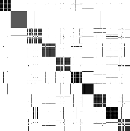
So when we apply it we get:

We exploit the fact that $X^\star$ has many repeated rows in our rounding step.

Approximation guarantees and tightness

A future post will focus on the mathematical analysis of this algorithm. In particular, the SDP is known to exactly recover the clusters when the points come from a data model called the stochastic ball model (see this and this). And it is known to approximate the centers when the points come from a mixture of subgaussian distributions.

About the interactive plots and clustering implementation

An implementation of the $k$-means SDP is available here. The implementation uses SDPNAL+ which is an amazing SDP solver for problems with non-negative constraints.

The first plot I wrote in javascript using D3. The second interactive plot I wrote in python using Bokeh. If someone asks I can write a tutorial on how to do these plots, but many tutorials and examples are available on the internet already.

Note that the fact that $X^\star$ has many repeated columns imply that many points are mapped to the same point after computing $PX^\star$. If you place the mouse on top of the points in the second plot you’ll see many images. But if you do it in the first one you’ll see one one (I added a little bit of noise so you can move the mouse and see a different image). That’s because I haven’t figured out how to replicate that behavior in javascript. I’ll be happy to hear suggestions.